Which algorithm you recommend? What accuracy it has? Why you measured accuracy the way you did?

#1. Properly load the data into Jupyter Notebooks

import matplotlib.pyplot as plt #matplotlib generates graphs.
import pandas as pd
from sklearn.datasets import load_iris
from sklearn.ensemble import GradientBoostingClassifier, RandomForestClassifier
from sklearn.svm import SVC #i.e. Support Vector Classifier
from sklearn.tree import DecisionTreeClassifier
from sklearn import tree
import graphviz
from sklearn.linear_model import LogisticRegression
from sklearn.svm import SVC
from sklearn import svm
from sklearn.linear_model import PassiveAggressiveClassifier
from sklearn.neighbors import RadiusNeighborsClassifier
from sklearn.model_selection import train_test_split
from sklearn.preprocessing import StandardScaler

data = pd.read_csv("crx.data", header=None)
print(data.columns)

Int64Index([0, 1, 2, 3, 4, 5, 6, 7, 8, 9, 10, 11, 12, 13, 14, 15], dtype='int64')

Change the column names to correspond to the “real” labels from the second link.

data.rename(columns={1 : "age", 
                     2 : "debt",
                     3 : "married",
                     4 : "bankcustomer", 
                     5 : "educationlevel", 
                     6 : "ethnicity",
                     7 : "yearsemployed", 
                     8 : "priordefault",
                     9 : "employed",
                     10 : "creditscore",
                     11 : "driverslicense",
                     12 : "citizen",
                     13 : "zipcode",
                     14 : "income",
                     15 : "approved"}, inplace=True)
print(data.head())

   0    age   debt married bankcustomer educationlevel ethnicity  \
0  b  30.83  0.000       u            g              w         v   
1  a  58.67  4.460       u            g              q         h   
2  a  24.50  0.500       u            g              q         h   
3  b  27.83  1.540       u            g              w         v   
4  b  20.17  5.625       u            g              w         v   

   yearsemployed priordefault employed  creditscore driverslicense citizen  \
0           1.25            t        t            1              f       g   
1           3.04            t        t            6              f       g   
2           1.50            t        f            0              f       g   
3           3.75            t        t            5              t       g   
4           1.71            t        f            0              f       s   

  zipcode  income approved  
0   00202       0        +  
1   00043     560        +  
2   00280     824        +  
3   00100       3        +  
4   00120       0        +  

Remove all question marks from value ‘age’, and convert it to numerical.

data.loc[83,'age'] = ""
data.loc[86,'age'] = ""
data.loc[92,'age'] = ""
data.loc[97,'age'] = ""
data.loc[254,'age'] = ""
data.loc[286,'age'] = ""
data.loc[329,'age'] = ""
data.loc[445,'age'] = ""
data.loc[450,'age'] = ""
data.loc[500,'age'] = ""
data.loc[515,'age'] = ""
data.loc[608,'age'] = ""



data['age'] = pd.to_numeric(data['age'])

#2. Summarize the data.Frequency tables for categorical variables and histograms for continuous variables.

%matplotlib inline
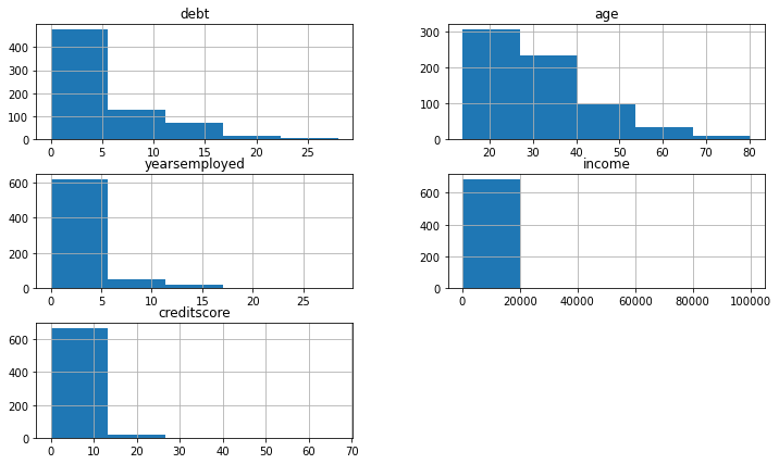
z = data.hist(column=['debt', 'age', 'yearsemployed', 'income', 'creditscore'],bins=5, figsize=(12,7))
print(z) #is not adding them i.e. it creates a longer list.

summary_data = data.describe()
print(summary_data)

#Categorical variables:
#             "married", 
#             "bankcustomer", 
#             'educationlevel', 
#             'ethnicity',  
#             'priordefault', 
#             'employed', 
#             'driverslicense',
#             'citizen',
#             'approved'

married = data.loc[:,"married"].value_counts()
print(married)

bankcustomer = data.loc[:,"bankcustomer"].value_counts()
print(bankcustomer)

educationlevel = data.loc[:,"educationlevel"].value_counts()
print(educationlevel)

ethnicity = data.loc[:,"ethnicity"].value_counts()
print(ethnicity)

priordefault = data.loc[:,"priordefault"].value_counts()
print(priordefault)

employed = data.loc[:,"employed"].value_counts()
print(employed)

driverslicense = data.loc[:,"driverslicense"].value_counts()
print(driverslicense)

approved = data.loc[:,"approved"].value_counts()
print(approved)

citizen = data.loc[:,"citizen"].value_counts()
print(citizen)

[[<AxesSubplot:title={'center':'debt'}>
  <AxesSubplot:title={'center':'age'}>]
 [<AxesSubplot:title={'center':'yearsemployed'}>
  <AxesSubplot:title={'center':'income'}>]
 [<AxesSubplot:title={'center':'creditscore'}> <AxesSubplot:>]]
              age        debt  yearsemployed  creditscore         income
count  678.000000  690.000000     690.000000    690.00000     690.000000
mean    31.568171    4.758725       2.223406      2.40000    1017.385507
std     11.957862    4.978163       3.346513      4.86294    5210.102598
min     13.750000    0.000000       0.000000      0.00000       0.000000
25%     22.602500    1.000000       0.165000      0.00000       0.000000
50%     28.460000    2.750000       1.000000      0.00000       5.000000
75%     38.230000    7.207500       2.625000      3.00000     395.500000
max     80.250000   28.000000      28.500000     67.00000  100000.000000
u    519
y    163
?      6
l      2
Name: married, dtype: int64
g     519
p     163
?       6
gg      2
Name: bankcustomer, dtype: int64
c     137
q      78
w      64
i      59
aa     54
ff     53
k      51
cc     41
m      38
x      38
d      30
e      25
j      10
?       9
r       3
Name: educationlevel, dtype: int64
v     399
h     138
bb     59
ff     57
?       9
j       8
z       8
dd      6
n       4
o       2
Name: ethnicity, dtype: int64
t    361
f    329
Name: priordefault, dtype: int64
f    395
t    295
Name: employed, dtype: int64
f    374
t    316
Name: driverslicense, dtype: int64
-    383
+    307
Name: approved, dtype: int64
g    625
s     57
p      8
Name: citizen, dtype: int64

Our data is skewed towards the left of the distribution because there are some outliers in our data, such as customers with a high income and credit score relative to the overall dataset. However, we are working with a limited number of data and it is still in the initial stage of development, we can leave it as-is for now. We can try to remove the outliers when we are tuning our model or when we have more data to work with.

#3. Split the sample into a test set and a train set with 20% of data being in the test dataset. Your random seed should be 808.

#split dataset into train and test, and set the random_state so it maintain the same result
data_features = data[['debt', "age", "married","bankcustomer", "educationlevel", "ethnicity", "yearsemployed", "priordefault","employed","creditscore",
"driverslicense","citizen","income"]]
data_target = data['approved']


x_train, x_test, y_train, y_test = train_test_split(data_features,
                                                    data_target,
                                                    test_size = 0.2,
                                                    random_state = 808)

#4. Try the following algorithms and choose the one that generates the best accuracy:

#First, we convert categorical variables to numerical.
data1 = pd.get_dummies(data).dropna()
print(data1)


print(list(data1.columns))

       age    debt  yearsemployed  creditscore  income  0_?  0_a  0_b  \
0    30.83   0.000           1.25            1       0    0    0    1   
1    58.67   4.460           3.04            6     560    0    1    0   
2    24.50   0.500           1.50            0     824    0    1    0   
3    27.83   1.540           3.75            5       3    0    0    1   
4    20.17   5.625           1.71            0       0    0    0    1   
..     ...     ...            ...          ...     ...  ...  ...  ...   
685  21.08  10.085           1.25            0       0    0    0    1   
686  22.67   0.750           2.00            2     394    0    1    0   
687  25.25  13.500           2.00            1       1    0    1    0   
688  17.92   0.205           0.04            0     750    0    0    1   
689  35.00   3.375           8.29            0       0    0    0    1   

     married_?  married_l  ...  zipcode_00720  zipcode_00760  zipcode_00840  \
0            0          0  ...              0              0              0   
1            0          0  ...              0              0              0   
2            0          0  ...              0              0              0   
3            0          0  ...              0              0              0   
4            0          0  ...              0              0              0   
..         ...        ...  ...            ...            ...            ...   
685          0          0  ...              0              0              0   
686          0          0  ...              0              0              0   
687          0          0  ...              0              0              0   
688          0          0  ...              0              0              0   
689          0          0  ...              0              0              0   

     zipcode_00928  zipcode_00980  zipcode_01160  zipcode_02000  zipcode_?  \
0                0              0              0              0          0   
1                0              0              0              0          0   
2                0              0              0              0          0   
3                0              0              0              0          0   
4                0              0              0              0          0   
..             ...            ...            ...            ...        ...   
685              0              0              0              0          0   
686              0              0              0              0          0   
687              0              0              0              0          0   
688              0              0              0              0          0   
689              0              0              0              0          0   

     approved_+  approved_-  
0             1           0  
1             1           0  
2             1           0  
3             1           0  
4             1           0  
..          ...         ...  
685           0           1  
686           0           1  
687           0           1  
688           0           1  
689           0           1  

[678 rows x 223 columns]
['age', 'debt', 'yearsemployed', 'creditscore', 'income', '0_?', '0_a', '0_b', 'married_?', 'married_l', 'married_u', 'married_y', 'bankcustomer_?', 'bankcustomer_g', 'bankcustomer_gg', 'bankcustomer_p', 'educationlevel_?', 'educationlevel_aa', 'educationlevel_c', 'educationlevel_cc', 'educationlevel_d', 'educationlevel_e', 'educationlevel_ff', 'educationlevel_i', 'educationlevel_j', 'educationlevel_k', 'educationlevel_m', 'educationlevel_q', 'educationlevel_r', 'educationlevel_w', 'educationlevel_x', 'ethnicity_?', 'ethnicity_bb', 'ethnicity_dd', 'ethnicity_ff', 'ethnicity_h', 'ethnicity_j', 'ethnicity_n', 'ethnicity_o', 'ethnicity_v', 'ethnicity_z', 'priordefault_f', 'priordefault_t', 'employed_f', 'employed_t', 'driverslicense_f', 'driverslicense_t', 'citizen_g', 'citizen_p', 'citizen_s', 'zipcode_00000', 'zipcode_00017', 'zipcode_00020', 'zipcode_00021', 'zipcode_00022', 'zipcode_00024', 'zipcode_00028', 'zipcode_00029', 'zipcode_00030', 'zipcode_00032', 'zipcode_00040', 'zipcode_00043', 'zipcode_00045', 'zipcode_00049', 'zipcode_00050', 'zipcode_00052', 'zipcode_00056', 'zipcode_00060', 'zipcode_00062', 'zipcode_00070', 'zipcode_00073', 'zipcode_00075', 'zipcode_00076', 'zipcode_00080', 'zipcode_00086', 'zipcode_00088', 'zipcode_00092', 'zipcode_00093', 'zipcode_00094', 'zipcode_00096', 'zipcode_00099', 'zipcode_00100', 'zipcode_00102', 'zipcode_00108', 'zipcode_00110', 'zipcode_00112', 'zipcode_00117', 'zipcode_00120', 'zipcode_00121', 'zipcode_00128', 'zipcode_00129', 'zipcode_00130', 'zipcode_00132', 'zipcode_00136', 'zipcode_00140', 'zipcode_00141', 'zipcode_00144', 'zipcode_00145', 'zipcode_00150', 'zipcode_00152', 'zipcode_00154', 'zipcode_00156', 'zipcode_00160', 'zipcode_00163', 'zipcode_00164', 'zipcode_00167', 'zipcode_00168', 'zipcode_00170', 'zipcode_00171', 'zipcode_00174', 'zipcode_00176', 'zipcode_00178', 'zipcode_00180', 'zipcode_00181', 'zipcode_00186', 'zipcode_00188', 'zipcode_00195', 'zipcode_00200', 'zipcode_00202', 'zipcode_00204', 'zipcode_00208', 'zipcode_00210', 'zipcode_00211', 'zipcode_00212', 'zipcode_00216', 'zipcode_00220', 'zipcode_00221', 'zipcode_00224', 'zipcode_00225', 'zipcode_00228', 'zipcode_00230', 'zipcode_00231', 'zipcode_00232', 'zipcode_00239', 'zipcode_00240', 'zipcode_00250', 'zipcode_00252', 'zipcode_00253', 'zipcode_00254', 'zipcode_00256', 'zipcode_00260', 'zipcode_00263', 'zipcode_00268', 'zipcode_00272', 'zipcode_00274', 'zipcode_00276', 'zipcode_00280', 'zipcode_00288', 'zipcode_00290', 'zipcode_00292', 'zipcode_00300', 'zipcode_00303', 'zipcode_00309', 'zipcode_00311', 'zipcode_00312', 'zipcode_00320', 'zipcode_00329', 'zipcode_00330', 'zipcode_00333', 'zipcode_00340', 'zipcode_00348', 'zipcode_00349', 'zipcode_00350', 'zipcode_00352', 'zipcode_00356', 'zipcode_00360', 'zipcode_00368', 'zipcode_00369', 'zipcode_00370', 'zipcode_00371', 'zipcode_00372', 'zipcode_00375', 'zipcode_00380', 'zipcode_00381', 'zipcode_00383', 'zipcode_00393', 'zipcode_00395', 'zipcode_00396', 'zipcode_00399', 'zipcode_00400', 'zipcode_00408', 'zipcode_00410', 'zipcode_00411', 'zipcode_00416', 'zipcode_00420', 'zipcode_00422', 'zipcode_00431', 'zipcode_00432', 'zipcode_00434', 'zipcode_00440', 'zipcode_00443', 'zipcode_00450', 'zipcode_00454', 'zipcode_00455', 'zipcode_00460', 'zipcode_00465', 'zipcode_00470', 'zipcode_00480', 'zipcode_00487', 'zipcode_00491', 'zipcode_00500', 'zipcode_00510', 'zipcode_00515', 'zipcode_00519', 'zipcode_00520', 'zipcode_00523', 'zipcode_00550', 'zipcode_00560', 'zipcode_00583', 'zipcode_00600', 'zipcode_00640', 'zipcode_00680', 'zipcode_00711', 'zipcode_00720', 'zipcode_00760', 'zipcode_00840', 'zipcode_00928', 'zipcode_00980', 'zipcode_01160', 'zipcode_02000', 'zipcode_?', 'approved_+', 'approved_-']

As before, we split the sample into a test set and a train set with 20% of data being in the test dataset. Your random seed should be 808. This needs to be done after the “get_dummies()” command for decision tree to work.

data_features = data1.loc[:,"age":"citizen_s"]
data_target = data1['approved_+']


x_train, x_test, y_train, y_test = train_test_split(data_features,
                                                    data_target,
                                                    test_size = 0.2,
                                                    random_state = 808)


print(x_train, x_test, y_train, y_test)

       age    debt  yearsemployed  creditscore  income  0_?  0_a  0_b  \
27   56.58  18.500         15.000           17       0    0    0    1   
100  37.50   1.750          0.250            0     400    0    0    1   
132  47.42   8.000          6.500            6   51100    0    1    0   
404  34.00   5.085          1.085            0       0    0    0    1   
401  28.92   0.375          0.290            0     140    0    0    1   
..     ...     ...            ...          ...     ...  ...  ...  ...   
480  16.92   0.500          0.165            6      35    0    1    0   
384  22.08  11.460          1.585            0    1212    0    0    1   
300  57.58   2.000          6.500            1      10    0    1    0   
249  21.83  11.000          0.290            6       0    0    0    1   
471  21.08   4.125          0.040            0     100    0    0    1   

     married_?  married_l  ...  ethnicity_z  priordefault_f  priordefault_t  \
27           0          0  ...            0               0               1   
100          0          0  ...            0               0               1   
132          0          0  ...            0               0               1   
404          0          0  ...            0               1               0   
401          0          0  ...            0               1               0   
..         ...        ...  ...          ...             ...             ...   
480          0          0  ...            0               1               0   
384          0          0  ...            0               1               0   
300          0          0  ...            0               1               0   
249          0          0  ...            0               0               1   
471          0          0  ...            0               1               0   

     employed_f  employed_t  driverslicense_f  driverslicense_t  citizen_g  \
27            0           1                 0                 1          1   
100           1           0                 0                 1          1   
132           0           1                 1                 0          1   
404           1           0                 0                 1          1   
401           1           0                 1                 0          1   
..          ...         ...               ...               ...        ...   
480           0           1                 0                 1          1   
384           1           0                 0                 1          1   
300           0           1                 1                 0          1   
249           0           1                 1                 0          1   
471           1           0                 1                 0          1   

     citizen_p  citizen_s  
27           0          0  
100          0          0  
132          0          0  
404          0          0  
401          0          0  
..         ...        ...  
480          0          0  
384          0          0  
300          0          0  
249          0          0  
471          0          0  

[542 rows x 50 columns]        age   debt  yearsemployed  creditscore  income  0_?  0_a  0_b  \
207  28.67  9.335          5.665            6     168    0    0    1   
406  40.33  8.125          0.165            2      18    0    1    0   
231  47.42  3.000         13.875            2    1704    0    1    0   
452  36.50  4.250          3.500            0      50    0    0    1   
567  25.17  2.875          0.875            0       0    0    1    0   
..     ...    ...            ...          ...     ...  ...  ...  ...   
457  29.67  0.750          0.040            0       0    0    0    1   
544  30.08  1.040          0.500           10      28    0    0    1   
145  32.83  2.500          2.750            6    2072    0    0    1   
342  26.92  2.250          0.500            0    4000    0    0    1   
323  48.58  0.205          0.250           11    2732    0    0    1   

     married_?  married_l  ...  ethnicity_z  priordefault_f  priordefault_t  \
207          0          0  ...            0               0               1   
406          0          0  ...            0               1               0   
231          0          0  ...            0               0               1   
452          0          0  ...            0               1               0   
567          0          0  ...            0               0               1   
..         ...        ...  ...          ...             ...             ...   
457          0          0  ...            0               1               0   
544          0          0  ...            0               0               1   
145          0          0  ...            0               0               1   
342          0          0  ...            0               1               0   
323          0          0  ...            0               0               1   

     employed_f  employed_t  driverslicense_f  driverslicense_t  citizen_g  \
207           0           1                 1                 0          1   
406           0           1                 1                 0          1   
231           0           1                 0                 1          1   
452           1           0                 1                 0          1   
567           1           0                 1                 0          1   
..          ...         ...               ...               ...        ...   
457           1           0                 1                 0          1   
544           0           1                 0                 1          1   
145           0           1                 1                 0          1   
342           1           0                 0                 1          1   
323           0           1                 1                 0          1   

     citizen_p  citizen_s  
207          0          0  
406          0          0  
231          0          0  
452          0          0  
567          0          0  
..         ...        ...  
457          0          0  
544          0          0  
145          0          0  
342          0          0  
323          0          0  

[136 rows x 50 columns] 27     1
100    0
132    1
404    0
401    0
      ..
480    0
384    0
300    0
249    1
471    0
Name: approved_+, Length: 542, dtype: uint8 207    1
406    0
231    1
452    0
567    1
      ..
457    0
544    0
145    1
342    0
323    1
Name: approved_+, Length: 136, dtype: uint8

data_features.info()

<class 'pandas.core.frame.DataFrame'>
Int64Index: 678 entries, 0 to 689
Data columns (total 50 columns):
 #   Column             Non-Null Count  Dtype  
---  ------             --------------  -----  
 0   age                678 non-null    float64
 1   debt               678 non-null    float64
 2   yearsemployed      678 non-null    float64
 3   creditscore        678 non-null    int64  
 4   income             678 non-null    int64  
 5   0_?                678 non-null    uint8  
 6   0_a                678 non-null    uint8  
 7   0_b                678 non-null    uint8  
 8   married_?          678 non-null    uint8  
 9   married_l          678 non-null    uint8  
 10  married_u          678 non-null    uint8  
 11  married_y          678 non-null    uint8  
 12  bankcustomer_?     678 non-null    uint8  
 13  bankcustomer_g     678 non-null    uint8  
 14  bankcustomer_gg    678 non-null    uint8  
 15  bankcustomer_p     678 non-null    uint8  
 16  educationlevel_?   678 non-null    uint8  
 17  educationlevel_aa  678 non-null    uint8  
 18  educationlevel_c   678 non-null    uint8  
 19  educationlevel_cc  678 non-null    uint8  
 20  educationlevel_d   678 non-null    uint8  
 21  educationlevel_e   678 non-null    uint8  
 22  educationlevel_ff  678 non-null    uint8  
 23  educationlevel_i   678 non-null    uint8  
 24  educationlevel_j   678 non-null    uint8  
 25  educationlevel_k   678 non-null    uint8  
 26  educationlevel_m   678 non-null    uint8  
 27  educationlevel_q   678 non-null    uint8  
 28  educationlevel_r   678 non-null    uint8  
 29  educationlevel_w   678 non-null    uint8  
 30  educationlevel_x   678 non-null    uint8  
 31  ethnicity_?        678 non-null    uint8  
 32  ethnicity_bb       678 non-null    uint8  
 33  ethnicity_dd       678 non-null    uint8  
 34  ethnicity_ff       678 non-null    uint8  
 35  ethnicity_h        678 non-null    uint8  
 36  ethnicity_j        678 non-null    uint8  
 37  ethnicity_n        678 non-null    uint8  
 38  ethnicity_o        678 non-null    uint8  
 39  ethnicity_v        678 non-null    uint8  
 40  ethnicity_z        678 non-null    uint8  
 41  priordefault_f     678 non-null    uint8  
 42  priordefault_t     678 non-null    uint8  
 43  employed_f         678 non-null    uint8  
 44  employed_t         678 non-null    uint8  
 45  driverslicense_f   678 non-null    uint8  
 46  driverslicense_t   678 non-null    uint8  
 47  citizen_g          678 non-null    uint8  
 48  citizen_p          678 non-null    uint8  
 49  citizen_s          678 non-null    uint8  
dtypes: float64(3), int64(2), uint8(45)
memory usage: 61.6 KB

data1.head()

	age	debt	yearsemployed	creditscore	income	0_?	0_a	0_b	married_?	married_l	...	zipcode_00720	zipcode_00760	zipcode_00840	zipcode_00928	zipcode_00980	zipcode_01160	zipcode_02000	zipcode_?	approved_+	approved_-
0	30.83	0.000	1.25	1	0	0	0	1	0	0	...	0	0	0	0	0	0	0	0	1	0
1	58.67	4.460	3.04	6	560	0	1	0	0	0	...	0	0	0	0	0	0	0	0	1	0
2	24.50	0.500	1.50	0	824	0	1	0	0	0	...	0	0	0	0	0	0	0	0	1	0
3	27.83	1.540	3.75	5	3	0	0	1	0	0	...	0	0	0	0	0	0	0	0	1	0
4	20.17	5.625	1.71	0	0	0	0	1	0	0	...	0	0	0	0	0	0	0	0	1	0

5 rows × 223 columns

#a. Decision Trees

from sklearn.tree import DecisionTreeClassifier
init_model = DecisionTreeClassifier ()
fitted_model = init_model.fit(x_train ,y_train)
test_predictions = fitted_model.predict(x_test)
accuracy_score = fitted_model.score(x_test,y_test)
print(accuracy_score)

#overall how many of the predictions are correct


#overall out of those defaults how many of those 0.17 are correct and not correct?

0.8455882352941176

#b. Logistic Regression

#Logistic regression
model_lr = LogisticRegression()
fitted_model_lr = model_lr.fit(x_train, y_train)
test_predictions_lr = fitted_model_lr.predict(x_test)
accuracy_lr = fitted_model_lr.score(x_test,y_test)
print(fitted_model_lr.coef_)
print(accuracy_lr)

#overall how many of the predictions are correct

[[ 4.84069824e-03 -2.46678805e-02  1.20267584e-01  1.64279116e-01
   5.13339863e-04 -7.02796069e-03 -1.76746656e-01 -2.76489739e-02
   1.08863388e-01  3.10703871e-02 -8.26650419e-02 -2.68692324e-01
   1.08863388e-01 -8.26650419e-02  3.10703871e-02 -2.68692324e-01
   1.08863388e-01 -9.05194758e-02 -9.94068100e-02  1.87520056e-01
  -2.93554456e-02  3.49157435e-02 -3.61569082e-01 -2.52229191e-01
  -9.00501443e-04 -2.10370142e-01 -8.76721486e-02  1.76003560e-01
  -5.84801526e-03  1.76604192e-01  2.42540281e-01  1.08863388e-01
  -1.29883594e-01 -2.29978369e-02 -3.51268838e-01  1.80746065e-01
   5.79890564e-02  1.89933137e-02 -1.73749301e-08 -9.58931264e-02
   2.20279985e-02 -1.72796178e+00  1.51653819e+00 -3.04359173e-01
   9.29355818e-02 -1.62785055e-03 -2.09795740e-01 -2.90778257e-01
   9.97707085e-02 -2.04160423e-02]]
0.8602941176470589

/Users/loizoskon/opt/anaconda3/lib/python3.9/site-packages/sklearn/linear_model/_logistic.py:763: ConvergenceWarning: lbfgs failed to converge (status=1):
STOP: TOTAL NO. of ITERATIONS REACHED LIMIT.

Increase the number of iterations (max_iter) or scale the data as shown in:
    https://scikit-learn.org/stable/modules/preprocessing.html
Please also refer to the documentation for alternative solver options:
    https://scikit-learn.org/stable/modules/linear_model.html#logistic-regression
  n_iter_i = _check_optimize_result(

#c. Bagging

#bagging, need to explore the concept and what each parameter does
from sklearn.ensemble import BaggingClassifier

#n_estimators is a number of randomly sampled datasets, similar to cv
model_bag = BaggingClassifier(
    base_estimator = tree.DecisionTreeClassifier(),
    n_estimators = 400,
    max_samples = 0.8,
    oob_score = True,
    random_state = 808)

fitted_model_bag = model_bag.fit(x_train,y_train)
test_predictions_bag = fitted_model_bag.predict(x_test)
accuracy_bag = fitted_model_bag.score(x_test,y_test)#validation accuracy, because I want to see if the model works generalize in new data
print(accuracy_bag)
print(model_bag.oob_score_)

0.8823529411764706
0.8616236162361623

#d. Boosting

from sklearn.ensemble import GradientBoostingClassifier, RandomForestClassifier

model_boost = GradientBoostingClassifier()

fitted_model_boost = model_boost.fit(x_train,y_train)
test_predictions_boost = fitted_model_boost.predict(x_test)
accuracy_boost = fitted_model_boost.score(x_test,y_test)
print(accuracy_boost)
print(model_boost)

0.8529411764705882
GradientBoostingClassifier()

#e. Random Forest

randomforest = RandomForestClassifier (random_state = 808)
model_randforest = RandomForestClassifier()

fitted_model_randforest = model_randforest.fit(x_train,y_train)
test_predictions_randforest = fitted_model_randforest.predict(x_test)
accuracy_randforest = fitted_model_randforest.score(x_test,y_test)
print(accuracy_randforest)

0.8382352941176471

#f. SVM

from sklearn.svm import SVC #i.e. Support Vector Classifier
svm=svm.SVC(random_state = 808)

print(svm.fit(x_train, y_train).score(x_test,y_test))

0.6985294117647058

#g. Passive Aggressive Classifier (Links to an external site.)

pa=PassiveAggressiveClassifier(random_state = 808)

print(pa.fit(x_train, y_train).score(x_test,y_test))

0.7573529411764706

#h. Radius Neighbors Classifier (Links to an external site.)

model_rn = RadiusNeighborsClassifier(radius=11700)
fitted_model_rn = model_rn.fit(x_train,y_train)
test_predictions_rn = fitted_model_rn.predict(x_test)
accuracy_rn = fitted_model_rn.score(x_test,y_test)
print(accuracy_rn)

0.6470588235294118

#5. After completing Step 4, explain: The accuracy of the algorithms above indicate the percentage of predictions that are actually correct. I would reccommend the bagging algorithm because it has the highest accuracy percentage (88,23%).

The confusion matrix below indicates that Bagging is the most suitable approach in reaching to the accuracy of the algorithms. In particular, the confusion matrix above shows us that the Bagging models have a higher number of true positives and true negatives than rest accuracy models. In this example above, we can see that bagging is compared with logistic regression and random forest classifiers, the 2nd and the 3rd highest accuracy models.

from sklearn.metrics import confusion_matrix

print('Confusion matrix: Bagging Classifiers')
print(confusion_matrix(y_test, test_predictions_bag))

print('Confusion matrix: Logistic Regression')
print(confusion_matrix(y_test, test_predictions_lr))

print('Confusion matrix: Random Forest Classifiers')
print(confusion_matrix(y_test, test_predictions_randforest))

Confusion matrix: Bagging Classifiers
[[75 12]
 [ 4 45]]
Confusion matrix: Logistic Regression
[[70 17]
 [ 2 47]]
Confusion matrix: Random Forest Classifiers
[[70 17]
 [ 5 44]]

6. Brief overview of the last two classifiers (Passive Agressive & Radius Neighbors).

Passive Agressive classifier is an online learning predictor best suited for systems that receive data in a continuous stream. The calculation passively corrects for the classifications and penalizes ‘aggressive’ for any miscalculation. While the model can perfectly predict all data, it will not change the algorithm; hence it is called passive. The term aggressive referst to the fact that when the model fails to predict the outcome variable just in the slightest, it will change the algorithm to compensate for the failed prediction for every set of a new sample of data.

Radius Neighbors classifer is similar to the KNN (k-nearest-neighbours) concept and makes predictions based on the data within a radius. Instead of locating the k-neighbors, the Radius Neighbors Classifier locates all examples in the dataset that are within a given radius of the new example. The radius neighbors are then used to make a prediction for the new example. The radius is defined in the feature space and generally assumes that the input variables are numeric and scaled to the range 0-1, e.g. normalized. The radius-based approach to locating neighbors is appropriate for those datasets where it is desirable for the contribution of neighbors to be proportional to the density of examples in the feature space.